We use MathJax
Measures of Central Tendency
A measure of central tendency is used when one intends to express the values in a distribution by a single representative value. Often, we refer to such a value as an average. Three types of average are quite common, the mean, the median, and the mode. It is necessary, though, to distinguish between population and sample data when computing averages.
Computing an Average from Raw Sample Data
Suppose we randomly sample twelve students who took the first statistics exam, and obtain the following raw data:
82, 76, 31, 87, 94, 76, 85, 88, 93, 98, 89, 93
- To find the mean, $\bar{x}$, of a sample of data, we use the formula $\bar{x} = \displaystyle\sum_{i=1}^n \dfrac{x_i}{n}$, where $n$ is the size of the sample. For this example, the mean is $\bar{x} = \dfrac{82+76+31+87+94+76+85+88+93+98+89+93}{12} \approx 82.67$ cm.
- To find the median of a sample of data, we put the data in order, and determine the value at position $\dfrac{n+1}{2}$ in the ordered data. If $n$ is odd, this position will be a specific value in the list. If $n$ is even, the formula will give a position and a half, which we interpret as being half way between two values in the list. For this example, the ordered data is 31, 76, 76, 82, 85, 87, 88, 89, 93, 93, 94, 98. The median occurs at position $\dfrac{12+1}{2}=6.5$, so the median occurs halfway between the sixth and seventh positions in the list. In other words,
$ \dfrac{87+88}{2} = 87.5$ cm is the median. There are many symbols in use for the median ($\tilde{x}$, $Q_2$, or $\operatorname{Med}$), but none of them is really common.
- To find the mode of a sample of data, we simply find the data value that occurs most often. However, it is possible that every value occurs equally often, in which case the mode does not exist. It is also possible that two (or more) values are tied for occurring most frequently, in which case two (or more) modes exist. For this example, the modes are 76 cm and 93 cm (which is most easily observed from the ordered list of data). Both of these values occur twice, while all other values occur less often.
Computing an Average from Raw Population Data
The essence of the computation is the same, whether the data came from a sample or a population. However, the variables used in the formulas are different, because of the interplay that occurs between populations and samples.
- The mean, $\mu$, of a population of data is given by the formula $\mu=\displaystyle\sum_{i=1}^N \dfrac{x_i}{N}$, where $N$ is the size of the population. It should be noted that not only do we have different variables for the mean ($\mu$ rather than $\bar{x}$), but also for the population size ($N$ rather than $n$).
- The median of a population will occur at position $\dfrac{N+1}{2}$ in the ordered data. Basically this is the same process, but the population size $N$ was used in place of the sample size $n$. When population and sample medians are discussed simultaneously, care should be taken to identify in words which quantity is being computed, as symbolism is not standardized.
- The mode of a population is computed in exactly the same way as the mode of a sample. Because the mode is extremely sensitive to small changes in values, it is rarely studied in the interplay of populations and samples, rendering moot the need for different symbols.
Estimating an Average from a Frequency Distribution
A big disadvantage occurs when working with data that has already been summarized in a frequency distribution. We no longer have the original raw data, and therefore we cannot use the original formulas for the various types of averages. The modifications we make to find averages in this case are at best estimates of the values that would be found from the raw data.
Suppose the heights of 169 freshmen at Western High School were found, and the results provided in the following table.
| Height |
Number of Students |
| 135-149 cm |
23 |
| 150-164 cm |
36 |
| 165-179 cm |
29 |
| 180-194 cm |
64 |
| 195-209 cm |
17 |
- To find the mean of this data, we first observe that we do not know the heights of any students, only their groupings into classes. So we use the class midpoints as the best estimate for the students in each class, and must take into account their frequencies. We use the weighted mean formula $\bar{x}=\dfrac{\displaystyle\sum_{i=1}^n w_i x_i}{\displaystyle\sum_{i=1}^n w_i}$, where $x_i$ is the midpoint of class $i$, and $w_i$ is the weight (or frequency) of that class. For this example, we estimate the mean to be $\bar{x}=\dfrac{142(23)+157(36)+172(29)+187(64)+202(17)}{23+36+49+44+17}=\dfrac{29308}{169} \approx 173.42$ cm. The computations may be more clear when laid out in a table, so we have added two columns to our example below.
| Height |
Class Midpoints
$x_i$ |
Number of Students
$w_i$ |
Product
$w_i x_i$ |
| 135-149 cm |
142 cm |
23 |
3266 |
| 150-164 cm |
157 cm |
36 |
5652 |
| 165-179 cm |
172 cm |
29 |
4988 |
| 180-194 cm |
187 cm |
64 |
11968 |
| 195-209 cm |
202 cm |
17 |
3434 |
| Totals |
|
169 |
29308 |
- To find the median of this data, we use $n=169$ and find position
$\dfrac{n+1}{2}=85$ in the list. The first two classes contain $23+36=59$ observations, and since $85-59=26$, position 85 is the 26th value in the third class. Since there are only 29 values in that class, it is certainly closer to the upper limit of the third class than to the lower limit, and we can interpolate to get an estimate:
$ 164.5+15\left(\dfrac{26-0.5}{29}\right)=177.7$ cm. Notice that we subtracted 0.5 in the numerator, which provides a linear interpolation under the assumption that the 29 data points were
evenly distributed between the class boundaries.
- To find the modal class of this data, we simply identify the class with the largest frequency. In this case, the modal class is the fourth class, 180-194 cm. We cannot actually find the mode itself without knowing the individual values.
Estimating an Average from a Graph
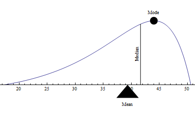
When estimating averages from a graph, imagine that the distribution is essentially a continuous function on a domain that extends from the minimum to the maximum values of the variable.
- The mean of the graph is located at the fulcrum of the area under the function. That is, imagine that the area under the graph was a solid uniform slab of an object, sitting on a children's see-saw. When the object would cause the see-saw to remain horizontal, then the mean will be at the fulcrum.
- The median is located where half of the area under the graph is to the left, and half is to the right.
- The mode of the graph is located at the value where the function reaches its maximum.

Characteristics of the Different Averages
The mean uses an algebraic formula, and that does make it easier to work with. That also means quantitative data is required; no mean is possible with only qualitative data. The mean is also the most stable average in sampling, in that a small change in any one data value cannot cause a large change in the average. However, the mean is easily influenced by outliers (data values quite unlike the great majority of values), and is in fact dependent on every value in the data set.
The median requires an ordering process rather than a straightforward formula, so its determination is not algebraic. Medians can be found on any data that is at least ordinal, which means some qualitative variables will have medians. The median is not influenced by outliers, nor most other values, in fact the only values which really count are those at the very center.
The mode does not require any structure on the data, so modes can be found even for nominal data. However, they may not exist, and if they do exist, they may not be unique.
Choosing an appropriate average for a set of data is not always easy. Suppose, for example, that the wages of a sample of 28 employees of a company are recorded, with the following results.
| Hourly wage |
Number of employees |
| $7.50 |
15 |
| $7.75 |
8 |
| $8.00 |
3 |
| $8.25 |
1 |
| $25.00 |
1 |
Note that the classes in this frequency distribution are precise, so our results will not involve estimates (beyond those due to any sampling process). When the three types of averages are computed, it can be found that the median and mode are both $\$7.50$, while the mean is slightly more than $\$8.27$. Now if the average wage was an issue in labor-management negotiations, management would not be happy hearing that the average was
$\$7.50$, since in fact that is the lowest wage they were paying. And labor would not be happy hearing that the average was almost $\$8.28$, since that would make all but one individual below average. None of the three averages really does a good job at representing the "center" of this set of data, and the basic cause of the problem is the presence of the outlier, $\$25.00$. If that value were excluded, the mean would drop to about $\$7.66$, well within the bulk of the data.

