
We use MathJax
Bivariate data involves a relationship between two random variables. When those variables are quantitative, each piece of data consists of an ordered pair of numbers. These values can be plotted on a graph (that is, a scatterplot), and inspected visually to see if there is a relationship. Often, data will have a linear trend, and linear regression is used to describe that trend.
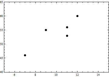
Suppose we sample five school-age boys, and determine their age in years and their height in inches. We want to determine if there is a relationship between age and height. The sample data is:
(7, 46), (9, 55), (11, 53), (11, 56), (12, 60)
Admittedly, this is a very small sample, but small samples allow us to more easily see the basic issues that need to be addressed. The scatterplot of the data follows.
From the data, we can easily compute some basic descriptive statistics for each variable.
But these statistics do not tell us anything about how the $x$ (age) and $y$ (height) variables might be related. For that, we need a different type of measure.
In some sense, we are interested in the spread of the data in two dimensions, as opposed to the one-dimensional measures we previously created. One of the measures of spread in one dimension was variance, defined (for a sample) to be $s^2 = \dfrac{ \sum\limits_{i=1}^n (x_i - \bar{x})^2}{n - 1}$. With a slight alteration, we can define a two-dimensional measure of spread called the covariance. As does the variance, it comes in two forms, one definition for a sample, and one for a population. And as with the variance, the reason is that the sample formula is an unbiased estimator of the population covariance.
| Population Formula | Sample Formula |
| $Cov(x,y) = \dfrac{ \sum\limits_{i=1}^N (x_i - \mu_x)(y_i - \mu_y)}{N}$ | $Cov(x,y) = \dfrac{ \sum\limits_{i=1}^n (x_i - \bar{x})(y_i - \bar{y})}{n - 1}$ |
If you compare the variance and covariance formulas, you see that quite often we are interested in the sum of the squared differences of data from the mean. These quantities are important enough to be identified with their own variable names. In general, the expression $S_{ab}$ means sum of the deviations of the product $ab$. More specifically, we have the following three quantities:
With these expressions, we could rewrite the sample variance and covariance.
Here are the computations that produce the covariance of our example above. The computation for each point takes a row of the table, and the last row of the table includes the totals for a few of the columns, including the values of $S_{xx}$, $S_{yy}$, and $S_{xy}$.
| $x_i$ | $y_i$ | $x_i - \bar{x}$ | $y_i - \bar{y}$ | $(x_i - \bar{x})^2$ | $(y_i - \bar{y})^2$ | $(x_i - \bar{x})(y_i - \bar{y})$ |
| 7 | 46 | $-3$ | $-8$ | 9 | 64 | 24 |
| 9 | 55 | $-1$ | 1 | 1 | 1 | $-1$ |
| 11 | 53 | 1 | $-1$ | 1 | 1 | $-1$ |
| 11 | 56 | 1 | 2 | 1 | 4 | 2 |
| 12 | 60 | 2 | 6 | 4 | 36 | 12 |
| $\overline{50}$ | $\overline{270}$ | $\overline{16}$ | $\overline{106}$ | $\overline{36}$ |
From this table, we see that $S_{xx} = 16$, $S_{yy} = 106$, and $S_{xy} = 36$. Together with the sum of the individual coordinates, we can easily determine the means, variances, standard deviations, and covariance.
We obtained a number for covariance, and we notice that it has units that are a product of the units for age and height. So how can we interpret this value? Below we have redrawn the scatterplot, and have included green lines indicating the means of each variable, and red lines from each point to the mean of each variable. The two green lines intersect at the point $(\bar{x},\bar{y})$, the point which has both average age and average height.
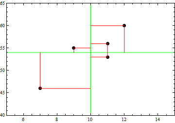
For each data point, the quantity $(x_i - \bar{x})(y_i - \bar{y})$ is the area of the rectangle formed by the two red lines, together with the green lines back to their intersection at $(\bar{x},\bar{y})$. So each value of $(x_i - \bar{x})(y_i - \bar{y})$ uses an "area" to measure how different a particular data point is from average. We notice that those points in the upper right and lower left regions will have a positive value for the "area" $(x_i - \bar{x})(y_i - \bar{y})$, while points in the upper left and lower right regions will have a negative value for the "area" $(x_i - \bar{x})(y_i - \bar{y})$. So if there are more points trending from lower left to upper right, the sum of the "areas" produced will be positive. And if there are more points trending from upper left to lower right, the sum of the "areas" produced will be negative.
The strange units for covariance make it somewhat difficult to interpret, since its value will depend on the scale used. We can remove this dependence on the scale by dividing by the standard deviation of each variable. This yields a quantity called the correlation.
| Population Formula | Sample Formula |
| $\rho = Corr(x,y) = \dfrac{ Cov(x,y) }{\sigma_x \sigma_y}$ | $r = Corr(x,y) = \dfrac{ Cov(x,y) }{ s_x s_y}$ |
All correlations satisfy the inequality $-1 \le r \le 1$. Correlations which are close to $-1$ or $1$ indicate a very strong linear relationship between the two variables. Correlations which are close to zero indicate essentially no linear relationship between the variables. Values falling between zero and the extremes are often stated to indicate a weak, moderate, or strong relationship. For our example, we found $r = \dfrac{9}{\sqrt{4} \sqrt{26.5}} = \dfrac{9}{\sqrt{106}} \approx 0.8741$, which would imply a rather strong positive relationship between age and height. Or in other words, as the age of a group of school boys increase, their heights also tend to increase.
Two alternative formulas for correlation are $r = \dfrac{ S_{xy} }{\sqrt{S_{xx} S_{yy}}}$ and $r = \dfrac{1}{n-1} \sum \limits_{i=1}^n \left( \dfrac{x_i-\bar{x}}{s_x} \right) \left(\dfrac{y_i-\bar{y}}{s_y} \right)$, both of which can be easily verified from the relationships given above. The second formula implies that correlation is an average z-score product of the data points.
Having determined that there is a trend, we could ask about the equation of the line that would best describe the trend. We would expect that such a line would give better estimates for our heights than simply using the mean height. In fact, in the scatterplot above, we can see that none of the data points fell on the horizontal line that represented the mean height. More explicitly, the "errors" or deviations (differences between the actual y-value and the y-value of the line) are rather large at the left and right ends of the data, as is shown in the scatterplot below.
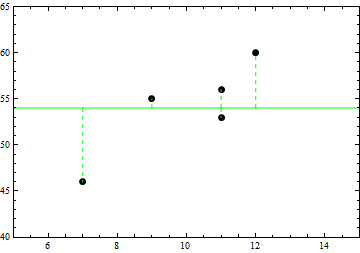
Could we draw a line which minimizes the errors? Our five points do not lie in a line, so we cannot draw a line for which all of the errors would be zero. And we need a way to deal with the five errors simultaneously. So we might consider minimizing the sum of the errors. As it turns out, it is quite possible to draw a line for which the sum of the errors is zero. Two such lines are illustrated below.
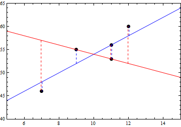
For the record, the two lines in the graph have the following equations.
We could easily verify that the sum of the errors in each case is zero. But doing so, or just by looking at the two lines and their errors, we might recognize the problem with our approach. Clearly, the red line was much less appropriate than the blue line, in spite of the fact that their sum was still zero, because its errors were each individually larger. That is because errors can be negative or positive, and the signs are what allow a sum of zero.
We could use absolute values of the errors. But you should recall that we encountered this issue before, when trying to define a measure of dispersion. Absolute values will omit signs, but they do have other algebraic complications. And in fact, when we discuss the estimation of populations from samples, we will find that they do not allow us to obtain the best estimators.
Therefore, we shall use the Least Squares Criterion to obtain our line. This criterion states that the sum of the squared errors (SSE) will be minimized. The line which satisfies the Least Squares Criterion will be unique, and it is called the regression line. The regression line is often called the line of best fit, which implies that the Least Squares Criterion is essentially the definition of what makes a best fit. For our example, the regression line has the equation $y=2.25 x + 31.5$, and is graphed in the next scatterplot.
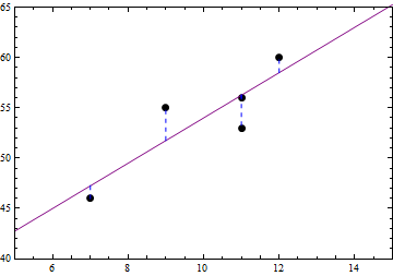
Visually, this line looks closer overall to the points, but the quantity that was minimized is not the sum of the errors, but rather the sum of the squared errors. Specifically, if $y_i$ are the y-values of the data points, and $\hat{y}_i$ are the values predicted by the regression line, then the sum of the squared errors (SSE) has the following formula.
| $SSE = \sum\limits_{i=1}^n (y_i - \hat{y}_i)^2$ |
Here are the numerical details for our example.
| Data Point | Point on Regression Line |
Error: $y_i - \hat{y}_i$ |
Squared Errors |
| (7, 46) | (7, 47.25) | $-1.25$ | 1.5625 |
| (9,55) | (9, 51.75) | $3.25$ | 10.5625 |
| (11,53) | (11, 56.25) | $-3.25$ | 10.5625 |
| (11,56) | (11, 56.25) | $-0.25$ | 0.0625 |
| (12,60) | (12, 58.5) | $1.5$ | 2.25 |
The sum of the squared errors (SSE) in our example is exactly 25, and this is the least possible value for this sum. For the record, the SSE of the red line was 194, the SSE of the blue line was 26, and the SSE for the green horizontal line was 106.
Now the green line represented the mean y-value, before we considered a non-horizontal trend. This "previous" SSE is usually called the total sum of the squares (abbreviated SST), and in fact is equivalent to $S_{yy}$. Using the regression line has been a substantial improvement over the mean, in fact it reduced the sum of the squared errors from 106 to 25, which is a 76.42% reduction. Or in other words, 76.42% of the variation in the heights is explained by the regression line. This quantity is called the coefficient of determination.
There are actually three quantities of the form SSQ, which we can describe as the sum of the squared "quantity Q". They are:
It should be noted that there are some relationships between these six quantities. Most notably:
Therefore, the coefficient of determination is the quantity $\dfrac{SSR}{SST} = \dfrac{S_{xy}^2}{S_{xx} S_{yy}} = r^2$. In other words, the coefficient of determination is the square of the correlation coefficient.
And finally, the formulas for the coefficients of the regression line $\hat{y} = \hat{\beta}_1 x + \hat{\beta}_0$ (and the coefficient of determination $r^2$) are:
| \begin{align} \hat{\beta}_1 &= \dfrac{S_{xy}}{S_{xx}} \\ \hat{\beta}_0 &= \bar{y} - \hat{\beta}_1 \bar{x} \\ r^2 &= \dfrac{S_{xy}^2}{S_{xx} S_{yy}} = \dfrac{SSR}{SST} \end{align} |
Typically, the sample coefficients of the regression equation are denoted $\hat{\beta}_1$ and $\hat{\beta}_0$, rather than $m$ and $b$ respectively, while the population coefficients are denoted $\beta_1$ and $\beta_0$. We should also note that the formula for $\hat{\beta}_0$ implies that the point $(\bar{x}, \bar{y})$ is a point on the regression line. In other words, the regression line passes through the intersection of the two averages.
For our example, the computations for these coefficients would be:
And for our regression line, we also have $SSE = 25$, $SST = 106$, and $SSR = 81$.
Suppose the data points are given by $(x_i, y_i)$, the regression line has the equation $\hat{y} = \hat{\beta}_1 x + \hat{\beta}_0$, so the points on the regression line are $(x_i,\hat{y}_i)$. Then we have
\begin{align} SSE &= \sum\limits_{i=1}^n (y_i - \hat{y}_i)^2 \\ &= \sum\limits_{i=1}^n (y_i - \hat{\beta}_1 x_i - \hat{\beta}_0)^2 \end{align}To minimize SSE is to find the values of $\hat{\beta}_1$ and $\hat{\beta}_0$ for which SSE is least, and we can do that through the use of derivatives and calculus. We shall first take a partial derivative with respect to $\hat{\beta}_0$ to find $\hat{\beta}_0$.
\begin{align} \frac{\partial}{\partial \hat{\beta}_0} \sum\limits_{i=1}^n (y_i - \hat{\beta}_1 x_i - \hat{\beta}_0)^2 &= \sum\limits_{i=1}^n \frac{\partial}{\partial \hat{\beta}_0} (y_i - \hat{\beta}_1 x_i - \hat{\beta}_0)^2 \\ &= \sum\limits_{i=1}^n (-2)(y_i - \hat{\beta}_1 x_i - \hat{\beta}_0) \end{align}Setting this quantity equal to zero leads to the following sequence of equations.
\begin{array}{c} \sum\limits_{i=1}^n (y_i - \hat{\beta}_1 x_i - \hat{\beta}_0) = 0 \\ \sum\limits_{i=1}^n y_i - \hat{\beta}_1 \sum\limits_{i=1}^n x_i - n \hat{\beta}_0 = 0 \\ \hat{\beta}_0 = \dfrac{\sum\limits_{i=1}^n y_i}{n} - \hat{\beta}_1 \dfrac{\sum\limits_{i=1}^n x_i}{n} \\ \hat{\beta}_0 = \bar{y} - \hat{\beta}_1 \bar{x} \end{array}Note that this argument also implies that for a regression line, the sum of the (unsquared) errors will be zero. That is, $\sum\limits_{i=1}^n (y_i - \hat{y}_i) = 0$.
A similar argument occurs when taking a partial derivative with respect to $\hat{\beta}_1$. However, we will substitute the result $\hat{\beta}_0 = \bar{y} - \hat{\beta}_1 \bar{x}$ to simplify the problem.
\begin{align} \frac{\partial}{\partial \hat{\beta}_1} \sum\limits_{i=1}^n (y_i - \hat{\beta}_1 x_i - \hat{\beta}_0)^2 &= \sum\limits_{i=1}^n \frac{\partial}{\partial \hat{\beta}_1} (y_i - \hat{\beta}_1 x_i - \bar{y} + \hat{\beta}_1 \bar{x})^2 \\ &= \sum\limits_{i=1}^n \frac{\partial}{\partial \hat{\beta}_1} ((y_i - \bar{y}) - \hat{\beta}_1 (x_i - \bar{x}))^2 \\ &= \sum\limits_{i=1}^n (-2)(x_i - \bar{x}) ((y_i - \bar{y}) - \hat{\beta}_1 (x_i - \bar{x})) \end{align}Setting this quantity equal to zero leads to the following sequence of equations.
\begin{array}{c} \sum\limits_{i=1}^n (x_i - \bar{x}) ((y_i - \bar{y}) - \hat{\beta}_1 (x_i - \bar{x})) = 0 \\ \sum\limits_{i=1}^n (x_i - \bar{x}) (y_i - \bar{y}) - \hat{\beta}_1 (x_i - \bar{x})^2 = 0 \\ \sum\limits_{i=1}^n (x_i - \bar{x}) (y_i - \bar{y}) = \sum\limits_{i=1}^n \hat{\beta}_1 (x_i - \bar{x})^2 \\ \hat{\beta}_1 = \dfrac{ \sum\limits_{i=1}^n (x_i - \bar{x}) (y_i - \bar{y}) }{ \sum\limits_{i=1}^n (x_i - \bar{x})^2 } \\ \hat{\beta}_1 = \dfrac{S_{xy}}{S_{xx}} \end{array}Before proceeding, we should also note that had we taken the derivative of the expression $\sum\limits_{i=1}^n (y_i - \hat{\beta}_1 x_i - \hat{\beta}_0)^2$ directly, then our work above would have found that $\sum\limits_{i=1}^n x_i (y_i - \hat{y}_i) = 0$, a result that we use below.
The equation $SST = SSR + SSE$ is an immediate result of the regression line having a zero sum of the errors.
\begin{align} SST &= \sum\limits_{i=1}^n (y_i - \bar{y})^2 \\ &= \sum\limits_{i=1}^n (y_i - \hat{y}_i + \hat{y}_i - \bar{y})^2 \\ &= \sum\limits_{i=1}^n (y_i - \hat{y}_i)^2 + 2 \sum\limits_{i=1}^n (y_i - \hat{y}_i)(\hat{y}_i - \bar{y}) + \sum\limits_{i=1}^n (\hat{y}_i - \bar{y})^2 \\ &= SSE + 2 \sum\limits_{i=1}^n (y_i - \hat{y}_i)(\hat{\beta}_1 x_i + \hat{\beta}_0 - \bar{y}) + SSR \\ &= SSE + 2 \hat{\beta}_1 \sum\limits_{i=1}^n x_i (y_i - \hat{y}_i) + 2(\hat{\beta}_0 - \bar{y}) \sum\limits_{i=1}^n (y_i - \hat{y}_i) + SSR \\ &= SSE + 2 \hat{\beta}_1 (0) + 2(\hat{\beta}_0 - \bar{y})(0) + SSR \\ &= SSE + SSR \end{align}And the derivation of the formula for SSR in terms of $S_{xy}$ and $S_{xx}$ (and therefore the connection between the coefficient of determination and the correlation coefficient) is as follows:
\begin{align} SSR &= SST - SSE \\ &= SST - \sum\limits_{i=1}^n (y_i - \hat{y}_i)^2 \\ &= SST - \sum\limits_{i=1}^n (y_i - \hat{\beta}_1 x_i - \hat{\beta}_0)^2 \\ &= SST - \sum\limits_{i=1}^n (y_i - \hat{\beta}_1 x_i - (\bar{y} - \hat{\beta}_1 \bar{x}))^2 \\ &= SST - \sum\limits_{i=1}^n (y_i - \bar{y} - \hat{\beta}_1 (x_i - \bar{x}))^2 \\ &= SST - \left( \sum\limits_{i=1}^n (y_i - \bar{y})^2 - 2 \hat{\beta}_1 \sum\limits_{i=1}^n (x_i - \bar{x})(y_i - \bar{y}) + \hat{\beta}_1 ^2 \sum\limits_{i=1}^n (x_i - \bar{x})^2 \right) \\ &= SST - (SST - 2 \hat{\beta}_1 S_{xy} + \hat{\beta}_1^2 S_{xx}) \\ &= 2 \left( \dfrac{S_{xy}}{S_{xx}} \right) S_{xy} - \left( \dfrac{S_{xy}}{S_{xx}} \right)^2 S_{xx} \\ &= \dfrac{S_{xy}^2}{S_{xx}} \end{align}Therefore $\dfrac{SSR}{SST} = \dfrac{S_{xy}^2}{S_{xx} S_{yy}} = r^2$.