We use MathJax
Random samples have variability. They can be quite unlike the population they were taken from, and this sampling error can cause us to make incorrect conclusions. This is a fact of statistical life, and we must learn how to live with it.
Members of a jury have the same problem as statisticians. They have been presented with a claim, and must rule on the truth of that claim. For the jury, the question is whether the individual is innocent (as he claims), or whether he is guilty. The evidence is presented, and the jury must then decide. There are two possible errors. The jury could mistakenly set a guilty individual free, or they could mistakenly send an innocent person to jail (or worse). In the American justice system, the benefit of the doubt goes to the individual on trial, who is assumed to be innocent until proven guilty (which requires agreement of all members of the jury).
Hypothesis testing is similar. A claim has been presented, and the statistician must rule on the truth of the claim. Is the claim true or not? The evidence is collected in the form of a sample, and the statistician must then decide. There are two possible errors. The statistician could mistakenly reject a true null hypothesis (called a Type I error), or mistakenly accept a false null hypothesis (called a Type II error). The benefit of the doubt goes to the null hypothesis, which is assumed to be true until the evidence seems to indicate otherwise. The situation is summarized in the following chart.
| $H_0$ is really true | $H_0$ is really false | |
| $H_0$ was rejected | Type I error | Correct conclusion |
| $H_0$ was accepted | Correct conclusion | Type II error |
Since there are two types of error, what are their respective probabilities of occurrence? The level of significance $\alpha$ is the probability of a Type I error. That is, $\alpha$ is the probability of rejecting a true null hypothesis. In our example above, that probability was 5%. Since the statistician chooses the level of significance, that value is under his control and typically kept small.
The graphs below show the relationship between a claim and the truth when the null hypothesis is true. Of course, that means the two distributions are identical.
| Claim (a true null hypothesis) Upper shaded area is the level of significance 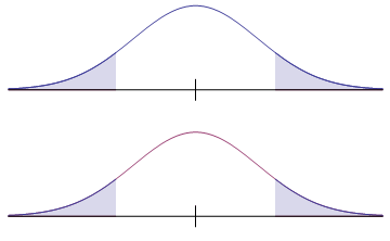
Truth Shaded area is the probability of a type I error |
The probability of a Type II error, which is the probability of accepting a false null hypothesis, is given by the value of $\beta$. That value is much harder to determine, because if the null hypothesis is false, then no information is available on what the population parameter value really is. If the null hypothesis was very different than the truth, the value of $\beta$ will be small. But if the null hypothesis was quite close to the truth, but off by just a little bit, then the value of $\beta$ could be quite large, and in fact as large as $1-\alpha$.
The two pairs of graphs below compare true distributions against claimed distributions, when a null hypothesis is false. In each case, the upper graph is the claim according to the null hypothesis, while the lower graph illustrates the truth. The value of $\beta$ is the shaded area in the lower graph.
| Claim (a very false null hypothesis) Upper shaded area is the level of significance 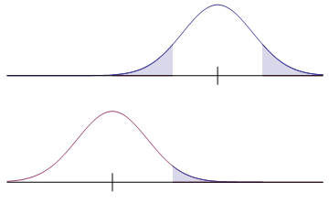 Truth Shaded area is the probability of a type II error |
Claim (a slightly false null hypothesis) Upper shaded area is the level of significance 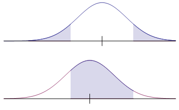 Truth Shaded area is the probability of a type II error |
So how can we control the probability of a Type II error? The options include:
The first option is actually quite common. By refusing to "accept" $H_0$, the Type II error becomes impossible. The language "fail to reject", and the contextual conclusion "there is insufficient evidence to conclude" indicate that the statistician has reached no conclusion on the matter. It is similar to the case of a hung jury that cannot decide.
The second option is more active. If "failing to reject" $H_0$ is not a suitable conclusion, the statistician could enlarge the sample. By doing so, the variation in the sample distribution is reduced, making it easier to identify a false null hypothesis that was actually close to the parameter of the actual distribution. However, if the null hypothesis is actually true, no ground will be gained through the use of this option.
The third option, the operating characteristic curve, gives possible values of $\beta$ as a function of the value of the unknown population parameter.
The third option uses an operating characteristic curve, often abbreviated as an OC curve. An OC curve gives the probability of accepting a null hypothesis for various possible parameter values, as was done in the two of the three pairs of graphs above. If the parameter sought is a population mean, then the steps for determining this probability are as follows.
To construct an OC curve, this process must be done for every possible alternative value of the mean.
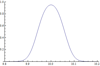
As an example, consider dog food that comes in 10-pound bags, and suppose it is known that the standard deviation of all dog food bags is 0.30 pounds. The statement of the weight on the bag leads to a null hypothesis claim of $\mu = 10$. Given that a sample of 100 bags is in the random sample, and a 5% level of significance is used, we would like to know the probability of accepting a false null hypothesis.
We begin by assuming the null hypothesis is true, so that $\mu = 10$. The critical values of the z-scores are $\pm z_{\alpha/2} = \pm \operatorname{invNorm}(0.025) = \pm 1.96$. Therefore, 95% of the samples should have mean weights in the interval determined by $X = \mu + z_{\alpha/2} \dfrac{\sigma}{\sqrt{n}} = 10 \pm 0.0588$, or in other words, between 9.9412 pounds and 10.0588 pounds.
So what if the true mean was $\mu = 9.95$ pounds? For this value, the null hypothesis would have been false (since 9.95 pounds is not 10 pounds), and we can find the probability that we would have accepted the false null hypothesis, thus committing a Type II error. For a true mean of 9.95 pounds, the z-scores for the values 9.9412 and 10.0588 pounds are then computed, and the probability determined.
\begin{align} z_1 &= \dfrac{9.9412 - 9.95}{0.3/\sqrt{100}} = -0.2933 \\ z_2 &= \dfrac{10.0588 - 9.95}{0.3/\sqrt{100}} = 3.6267 \\ P(-0.2933 < z < 3.6267) &= \operatorname{normalcdf}(-0.2933,3.6267) = 0.6152 \end{align}To obtain an OC curve, this process must be done for every possible alternative mean. That is, we replace 9.95 with $\mu$ in the above computations. We need to find
\begin{equation} P\left( \dfrac{9.9412 - \mu}{0.3/\sqrt{100}} < z < \dfrac{10.0588 - \mu}{0.3/\sqrt{100}} \right) \end{equation}as a function of the value $\mu$. We obtain the following graph for the values of $\beta$, the probability of a type II error.
Based on the construction of our example, we can produce an algebraic formula. Suppose a population has a true mean of $\mu$, a population standard deviation of $\sigma$, from which samples of size $n$ are randomly selected. Also suppose that $\mu_0$ is the claimed mean in the null hypothesis, and the level of significance is $\alpha$. Then the z-scores are computed by
\begin{gather} z = \dfrac{ \mu_0 \pm z_{\alpha/2} \dfrac{\sigma}{\sqrt{n}} - \mu }{\dfrac{\sigma}{\sqrt{n}}} \\ \dfrac{ \mu_0 - z_{\alpha/2} \dfrac{\sigma}{\sqrt{n}} - \mu }{\dfrac{\sigma}{\sqrt{n}}} < z < \dfrac{ \mu_0 + z_{\alpha/2} \dfrac{\sigma}{\sqrt{n}} - \mu }{\dfrac{\sigma}{\sqrt{n}}} \\ -z_{\alpha/2} + \dfrac{\mu_0 - \mu}{\sigma/\sqrt{n}} < z < z_{\alpha/2} + \dfrac{\mu_0 - \mu}{\sigma/\sqrt{n}} \end{gather}Therefore, the formula for $\beta$ as a function of the true mean $\mu$ is given by
| $\beta = P\left( -z_{\alpha/2} + \dfrac{\mu_0 - \mu}{\sigma/\sqrt{n}} < z < z_{\alpha/2} + \dfrac{\mu_0 - \mu}{\sigma/\sqrt{n}} \right)$ |
This formula, or its derivation, may be easily modified to handle situations when $s$ is used as an estimate for $\sigma$, or when the hypothesis is one-tailed, or when the OC curve for a different population parameter is sought.