Discrete Uniform Distributions

A random variable has a uniform distribution when each value of the random variable is equally likely, and values are uniformly distributed throughout some interval. Uniform distributions can be discrete or continuous, but in this section we consider only the discrete case.

The Formulas

If $X$ is uniformly distributed on the set $\{1, 2, 3, ..., N\}$, then the following formulas apply.

\begin{align} P(x) &= \dfrac{1}{N} \\ M(t) &= \dfrac{ e^t (1 - e^{tN})}{N (1 - e^t)} \\ E(X) &= \dfrac{N+1}{2} \\ Var(X) &= \dfrac{N^2-1}{12} \end{align}

If $Y$ is uniformly distributed on the set $\{a, a+k, a+2k, ..., b\}$, then the following formulas apply.

\begin{align} P(y) &= \dfrac{k}{b-a+k} \\ M(t) &= \dfrac{ e^{at} (1-e^{ktN})}{N (1-e^{kt})} \\ E(Y) &= \dfrac{a+b}{2} \\ Var(Y) &= k^2 \left(\dfrac{N^2-1}{12}\right) \end{align}

Rolling One Die

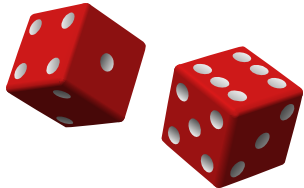
An example of a discrete uniform distribution on the first N integers is the statistical experiment of rolling one die, where the random variable $X$ represents the outcome of the die. For the standard six-sided die, we have the probability $P(X)=\frac16$ for each outcome. Furthermore, the expected value is $E(X)=\dfrac{6+1}{2} = 3.5$, so over the long run, the average of the outcomes should be midway between 3 and 4. We also find that the variance is $Var(X) = \dfrac{6^2-1}{12} = \dfrac{35}{12} \approx 2.9167$, and the standard deviation of the outcomes is $\sigma_X = \sqrt{\dfrac{35}{12}} \approx 1.7078$.

Derivation of the First Case

When we begin with the set $\{1, 2, 3, ..., N\}$, we clearly have $N$ possible outcomes, and since each is equally likely, we have $P(x)=\dfrac{1}{N}$.

The moment generating function is found by evaluating $E(e^{tX})$. We recognize the sum that results as a sum of a geometric series.

\begin{align} M(t) &= E(e^{tx}) = \sum\limits_{x=1}^N e^{tx} \dfrac1N \\ &= \dfrac1N \sum\limits_{x=1}^N (e^t)^x \\ &= \dfrac1N e^t \dfrac{1-e^{tN}}{1-e^t} \\ &= \dfrac{e^t (1 - e^{tN}}{N (1 - e^t)} \end{align}

The function $M(t)$ could be used to find the expected value and the variance, but the algebra is ugly, the result actually has the indeterminate form $\dfrac00$, and L'Hopital's Rule would be needed to evaluate the limit of the expression as $t$ approaches zero. So instead, we use the basic definitions of $E(X)$, $E(X^2)$, and $Var(X)$. In the following derivations, we will need to use two results from calculus. The sum of the first $N$ integers is given by $\sum\limits_{x=1}^N x = \dfrac{N(N+1)}{2}$, and the sum of the first $N$ squares is given by $\sum\limits_{x=1}^N x^2 = \dfrac{N(N+1)(2N+1)}{6}$.

Now the expected value formula is derived as follows.

\begin{align} E(X) &= \sum x P(x) \\ &= \sum\limits_{x=1}^N x \dfrac{1}{N} \\ &= \dfrac{1}{N} (1 + 2 + 3 + \cdots + N) \\ &= \dfrac{1}{N} \left[ \dfrac{N(N+1)}{2}\right] \\ &= \dfrac{N+1}{2} \end{align}

Before we can produce the variance formula, we first need a formula for $E(X^2)$.

\begin{align} E(X^2) &= \sum x^2 P(x) \\ &= \sum\limits_{x=1}^N x^2 \dfrac{1}{N} \\ &= \dfrac{1}{N} (1^2 + 2^2 + 3^2 + \cdots + N^2) \\ &= \dfrac{1}{N} \left[ \dfrac{N(N+1)(2N+1)}{6}\right] \\ &= \dfrac{(N+1)(2N+1)}{6} \end{align}

Now we can obtain the variance formula.

\begin{align} Var(X) &= E(X^2)-(E(X))^2 \\ &= \dfrac{(N+1)(2N+1)}{6} - \left( \dfrac{N+1}{2} \right)^2 \\ &= \dfrac{2N^2 + 3N+1}{6} - \dfrac{N^2+2N+1}{4} \\ &= \dfrac{N^2-1}{12} \end{align}

Of course, this implies that the standard deviation of a discrete uniform distribution is given by $\sigma = \sqrt{ \dfrac{N^2-1}{12}}$.

Derivation of the General Case

The set $\{a, a+k, a+2k, ..., b\}$ is a generalization of the first case, where we no longer require the minimum value to be 1, nor the spacing between values to be 1. We observe that the size of the sample space is $N = \dfrac{b-a}{k}+1 = \dfrac{b-a+k}{k}$. Therefore, the probability of each outcome is given by $P(y)=\dfrac{k}{b-a+k}$.

Now, we shall relate the random variable $Y$ on this set with the random variable $X$ on the set $\{1, 2, 3, ..., N\}$. The equation relating these two random variables is given by $Y= kX + (a-k)$, and it is a linear relationship. Therefore, we can use transformations to find the moment generating function, the expected value, and the variance.

For the moment generating function, we use the result $M_{aX+b}(t) = e^{tb} M_X(at)$. We get

\begin{align} M_Y(t) &= M_{kX+(a-k)}(t) \\ &= e^{t(a-k)} M_X(kt) \\ &= e^{t(a-k)} \dfrac{e^{kt} (1-e^{ktN})}{N (1-e^{kt})} \\ &= \dfrac{ e^{at} (1-e^{ktN})}{N (1-e^{kt})} \end{align}

The derivation of the expected value formula is as follows:

\begin{align} E(Y) &= E(kX + (a-k)) \\ &= k E(X) + (a-k) \\ &= k\left(\dfrac{N+1}{2}\right) + (a-k) \\ &= \dfrac{k}{2} \left( \dfrac{b-a+k}{k} + 1\right) + a-k \\ &= \dfrac{a+b}{2} \end{align}

And the derivation of the variance formula is even easier.

\begin{align} Var(Y) &= Var(kX + (a-k)) \\ &= k^2 Var(X) \\ &= k^2 \left(\dfrac{N^2-1}{12}\right) \end{align}

Epilogue

During the Second World War, the Allied forces wanted to estimate the number of tanks placed in the field by the other side. Since the tanks were conveniently numbered, they formed a discrete uniform distribution. The allies had a sample of numbers, so they could determine a sample minimum, a sample maximum, and an average gap between the numbers. From these, they could estimate a population size.