Empirical Probability

Probability is the mathematical study of measuring uncertainty. Probabilities are empirically determined when their numerical values are based upon a sample or a census of data giving a distribution of events.

The Basic Rule

When examined empirically, the probability that an event will occur will be equal to the percentage of times it did occur in a sample or census. More specifically, if $A$ is the name of an event, $f$ is the frequency with which that event occurred, and $n$ is the sample size, then:

$P(A) = \dfrac{f}{n}$

Probabilities from a Frequency Distribution

Suppose a sample of 400 households with children was obtained, and the number of children under age 18 in each household was counted. The following frequency distribution gives the data from the sample.

Number of Children	Number of Households
1	92
2	156
3	108
4	28
5	12
6	4

Suppose one household was randomly selected. We will let $C$ represent the number of children. Then:

The probability that the household contained exactly 4 children is:
$P(C=4)=\dfrac{28}{400}=0.07$.
The probability that the household contained more than 4 children is:
$P(C > 4) = P(C=5)+P(C=6) = \dfrac{12}{400} + \dfrac{4}{400} = \dfrac{16}{400} = 0.04$.
The probability that the household contained at least 4 children is:
$P(C \geq 4) = P(C=4)+P(C=5)+P(C=6) = \dfrac{28}{400} + \dfrac{12}{400} + \dfrac{4}{400} = \dfrac{44}{400} = 0.11$.
The probability that the household contained less than 4 children is:
$P(C < 4) = P(C=1) + P(C=2) + P(C=3) = \dfrac{92}{400} + \dfrac{156}{400} + \dfrac{108}{400} = \dfrac{356}{400} = 0.89$.
The probability that the household contained at most 4 children is:
$P(C \leq 4) = P(C=1) + P(C=2) + P(C=3) + P(C=4) \vphantom{\dfrac12}$
$= \dfrac{92}{400} + \dfrac{156}{400} + \dfrac{108}{400} + \dfrac{28}{400} = \dfrac{384}{400} = 0.96$.
The probability that the household did not contain exactly 4 children is:
$P(C \ne 4) = P(C=1) + P(C=2) + P(C=3) + P(C=5)+P(C=6) \vphantom{\dfrac12}$
$ = \dfrac{92}{400} + \dfrac{156}{400} + \dfrac{108}{400} + \dfrac{12}{400} + \dfrac{4}{400} = \dfrac{372}{400} = 0.93$.
The probability that the household contained between 2 and 5 children, inclusive, is:
$P(2 \leq C \leq 5) = P(C=2) + P(C=3) + P(C=4) + P(C=5) \vphantom{\dfrac12}$
$ = \dfrac{156}{400} + \dfrac{108}{400} + \dfrac{28}{400} + \dfrac{12}{400} = \dfrac{304}{400} = 0.76$.
The probability that the household contained 4 or 5 children is:
$P(C=4 \text{ or } C=5) = P(C=4) + P(C=5) = \dfrac{28}{400} + \dfrac{12}{400} = \dfrac{40}{400} = 0.10$.
The probability that the household contained 4 and 5 children is:
$P(C=4 \text{ and } C=5) = 0$,
because a single household either has 4 children, or it has 5 children, but it cannot have both simultaneously.

The basic rule was used in almost all parts of the preceding example. Notice especially how important the "little" words were. Be sure you understand what "at most" and "at least" mean. Also notice the distinction between "and" and "or".

The last part of the example, where we looked for a household that had both 4 and 5 children, turned out to have a probability of zero. We call the events "having 4 children" and "having 5 children" mutually exclusive events, which means they cannot happen simultaneously. Usually, the classes in a frequency distribution will be constructed so that they are mutually exclusive.

Probabilities from Multivariate Data

Suppose a sample of 2000 individuals found 1700 who had health insurance, 920 were young (age at most 35 years), and 750 were both young and insured.

This particular example involves two independent variables for each subject, their age, and whether or not they are insured. We need to organize this data to help determine any probability questions that may arise from it. In particular, we shall show three techniques for organizing it, the contingency table, the Venn diagram, and the tree diagram.

Contingency tables are two-dimensional, allowing data to be classified according to two different independent variables. One variable is displayed in columns, and the other in rows. For each variable, we do need to identify all possible values of that variable. For our example, the values for age are "young" and "not young", while the values for insured status are "insured" and "not insured". In the table below, we have included the original data values in bold. The other values were obtained through subtraction, since we know that each row and column must give the total at the right or bottom.

	Insured	Not Insured	Totals
Young	750	170	920
Not Young	950	130	1080
Totals	1700	300	2000

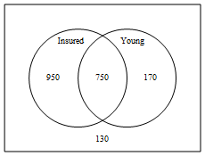
A Venn diagram consists of a rectangular region representing the entire sample, and one circular subset for each independent variable. The variable must be Boolean, in that there are only two possible values for the variable, such as true or false, yes or no, exists or does not exist, etc. Each circle must overlap every other circle. In the Venn diagram below, we began by entering the value 750 for the intersection of the two circles (for individuals who were both young and insured). We subtracted this value from each of the individual frequencies to obtain the non-intersected portion of each circle. Lastly, we subtracted the three quantities from the total sample size to obtain the value for the rectangle outside of the two circles.

A tree diagram consists of a column of branches for each independent variable. Since we have two independent variables, our tree will have two columns. We have chosen to put the variable "insured status" first, and there are two possible values for it, so the first column has two branches. The second variable also has two possible values ("young" and "not young"), so for each value in the first column, there are two more branches in the second column. In each column, the numbers must add to the sample size (in this case 2000). We must be careful in the second column, where each branch represents particular values for both insured status and age. Appropriate subtractions are used to determine these values.

Having organized the data, let's consider a few probability questions. Suppose one person was randomly selected from the original sample of 2000 individuals.

The probability that the person was insured is:
$P(\text{insured}) = \dfrac{1700}{2000} = 0.85$.
The probability that the person was young and insured is:
$P(\text{young and insured}) = \dfrac{750}{2000} = 0.375$.
The probability that the person was insured but not young is:
$P(\text{insured and not young}) = \dfrac{950}{2000} = 0.475$.
The probability that the person was young or insured is:
$P(\text{young or insured}) = \dfrac{750}{2000} + \dfrac{950}{2000} + \dfrac{170}{2000} = \dfrac{1870}{2000} = 0.935$.

You should notice that each of the three approaches laid out all of the values needed, so that the computation of any collection of events could be done simply by identifying the appropriate values to add.

Comparing these three approaches, we see benefits and disadvantages for each. The contingency table was limited to two variables, since it only has two dimensions. (A three-dimensional table would require writing inside of block of Swiss cheese, or something similar). Venn diagrams will work for both two and three variables, but to progress beyond three variables non-circular regions would be needed. A tree diagram can be drawn for any number of variables, although it does get large and cumbersome.

The type of variable used in each diagram differs as well. The Venn diagram is restricted to Boolean variables, those that have only two possible values each. The contingency table and the tree diagram allow many possible values for each variable. However, the variable does still have to be discrete.