
We use MathJax
Recursion is the process by which a previous result is used as the input for the next result. In the recursive formulas of sequences we have seen so far, this fact was evidenced when $a_{n-1}$ was used to find $a_n$.
The simplest recursive formulas produce arithmetic and geometric sequences. Specifically, $a_n=a_{n-1}+d$ produces an arithmetic sequence whose explicit formula is $a_n=a_1+d(n-1)$. And $a_n=r(a_{n-1})$ produces a geometric sequence whose explicit formula is $a_n=a_1 r^{n-1}$. More information on these sequences may be found on the pages Arithmetic Sequences and Geometric Sequences.
A recursive formula that is linear in its previous term also produces a fairly simple case. Specifically, $a_n=ca_{n-1}+d$ will produce the case where the ratios of differences is common, and its explicit formula is $a_n=\left(\dfrac{d}{c-1}+a_1\right)c^{n-1}-\dfrac{d}{c-1}$. Note that the explicit formula is the sum of an exponential term with a constant term. See the web page Recognizing More Patterns for more information.
The repetition of any single operation is also a fairly simple case. For example, the sequence $a_n={a_{n-1}}^p$ will produce the explicit formula $a_n={a_1}^{p^{n-1}}$, where the variable is in the exponent of the exponent. As an example, the recursive formula $a_n={a_{n-1}}^2, \quad a_1=3$ produces the sequence $3, 9, 81, 6561, \ldots$ When written with exponents as $3, 3^2, 3^4, 3^8, \ldots$, the pattern is more visible.
However, even quite simple recursive formulas can produce some exotic behavior. The formulas certainly provide a mechanical approach to obtaining values of the function, but the basic characteristic of a sequence's eventual behavior is not readily apparent through a multitude of values. The cobweb diagram gives a pictorial approach to this problem.
To draw a cobweb diagram for the recursive formula $a_n=f(a_{n-1})$, proceed as follows.
Let us consider the cobweb diagrams for some simple cases, and their resulting graphs. Here are two diagrams for the sequence $a_n=\frac12 a_{n-1}+2$. In both of these diagrams, the slope of the recursive function is less than one, and the iterations of the cobweb are approaching the intersection of the function with the line $y=x$. This sequence is converging to the value 4, the solution of the equation $x=f(x)$. The equation $x=f(x)$ is called the fixed-point equation, and its solution is a fixed point of the recursive equation. If the first term of the sequence was the solution of the fixed-point equation, then the sequence would have been constant.
\begin{align}
a_n &= \frac12 a_{n-1}+2 \\ a_1 &= 0.3
\end{align}
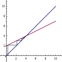
\begin{multline} 0.3, 2.15, 3.075, 3.538, 3.769, 3.884, \ldots \\ \ldots, 3.9995, 3.9998, 3.9999, \ldots \end{multline} 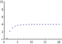 |
\begin{align}
a_n &= \frac12 a_{n-1}+2 \\ a_1 &= 7
\end{align}
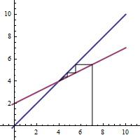
\begin{multline} 7, 5.5, 4.75, 4.375, 4.188, \ldots \\ \ldots, 4.0007, 4.0004, 4.0002, \ldots \end{multline} 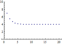 |
Here are two diagrams for the sequence $a_n=2a_{n-1}-4$. In these diagrams, the slope of the recursive function is greater than one, and the iterations of the cobweb are diverging from the intersection of the function with the line $y=x$. The values of this sequence are unbounded.
\begin{align}
a_n &= 2a_{n-1}-4 \\ a_1 &= 3.8
\end{align}
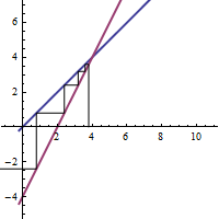
\begin{equation*} 3.8, 3.6, 3.2, 2.4, 0.8, -2.4, -8.8, -21.6, \ldots \end{equation*} 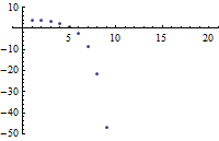 |
\begin{align}
a_n &= 2a_{n-1}-4 \\ a_1 &= 4.2
\end{align}
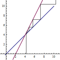
\begin{equation*} 4.2, 4.4, 4.8, 5.6, 7.2, 10.4, 16.8, 29.6, \ldots \end{equation*}  |
Here are the cobweb diagrams of three related equations. In the first, we see that cyclic behavior is possible, while the second and third graphs demonstrate that small changes in the equation can cause the iterations to either approach or diverge from the fixed point.
\begin{align}
a_n &= \frac{2}{a_{n-1}} \\ a_1 &= 0.8
\end{align}
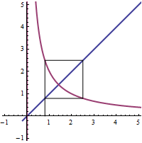
\begin{equation*} 0.8, 2.5, 0.8, 2.5, 0.8, 2.5, \ldots \end{equation*} 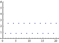
|
\begin{align}
a_n &= \frac{2}{a_{n-1}}-0.1 \\ a_1 &= 0.8
\end{align}
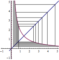
\begin{equation*} 0.8, 2.4, 0.733, 2.627, 0.661, 2.925, \ldots \end{equation*} 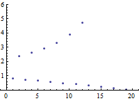
|
\begin{align}
a_n &= \frac{2}{a_{n-1}}+0.1 \\ a_1 &= 0.8
\end{align}
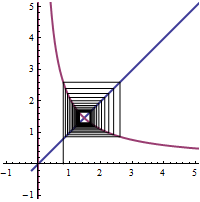
\begin{equation*} 0.8, 2.6, 0.869, 2.401, 0.933, 2.244, \ldots \end{equation*} 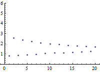
|
The eventual behavior of a sequence can also be quite unpredictable. Although the values of the sequence pictured below are completely determined by the recursive formula and are clearly bounded, yet they do not converge to a fixed point, nor are they cyclic. In fact, except for the fact that all of the values are between zero and one, the long-run behavior of this system appears quite chaotic.
\begin{align}
a_n &= 3.88a_{n-1}(1-a_{n-1}) \\ a_1 &= 0.17
\end{align}
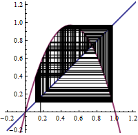
\begin{equation*} 0.17, 0.55, 0.96, 0.14, 0.48, 0.97, \ldots \end{equation*} 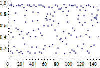
|
Arithmetic sequences can only show one type of end behavior, unboundedness (unless the common difference is zero). Geometric sequences can be either unbounded, or converge to a fixed point. Neither arithmetic nor geometric sequences will show cyclic or chaotic behavior. The classic example of a sequence that shows all of these end behaviors is the logistic sequence. For more information, see the web page Logistic Sequences.